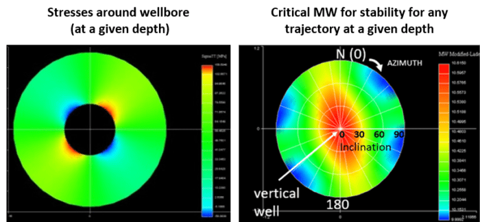
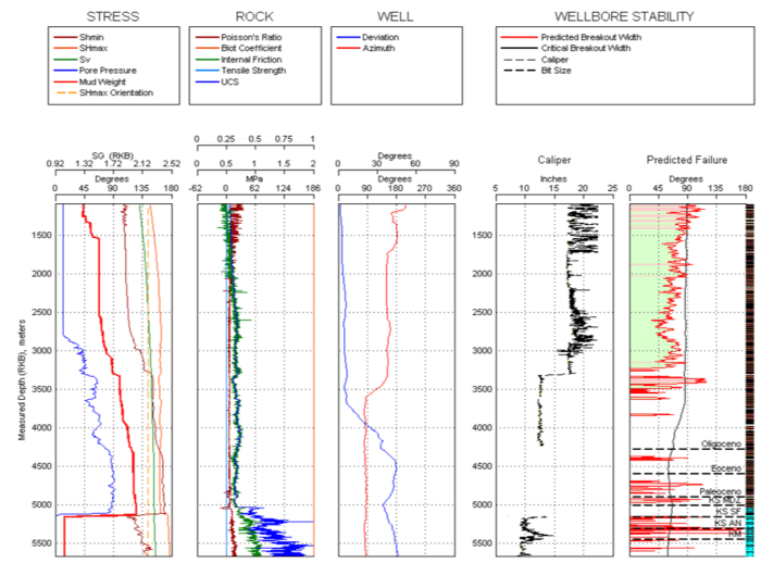
A 1D geomechanical model (again, consisting of stress magnitudes and orientation, pressure and mechanical properties) is constructed from wellbore data, along the path of that wellbore and is used to quantify stresses (magnitudes and orientation), rock mechanical properties (deformability and strength) and pore pressure local to that wellbore. These data are typically presented as log traces of the given parameter, e.g., Sv, Shmax, Shmin, Young’s modulus, Poisson’s ratio, UCS (Unconfined Compressive Strength) and friction angle, as a function of depth (most often ft-TVD or m-TVD). Whenever possible, the 1D geomechanical model results are calibrated to, using a wellbore stability model, reproduce the failure events observed in the wells.
At OFG, we build and calibrate the 1D geomechanical model for our projects following state-of-the-practice workflows and state-of-the-art tools (proprietary and commercial) with information gathered from well logs (e.g., GR, sonic, density, resistivity, image, and caliper); injectivity test data (e.g., DFITS, mini-fracs, LOTs, XLOTs, Step rate tests, and well testing); rock mechanics laboratory data (e.g., from cores and analogs); pore pressure data (e.g., from logs, RFTs, and MDTs); and drilling data (e.g., WOB, ROP, cavings).
Drilling Event Analysis
A necessary step in building a calibrated 1D geomechanical model is to perform the Drilling Event Analysis.
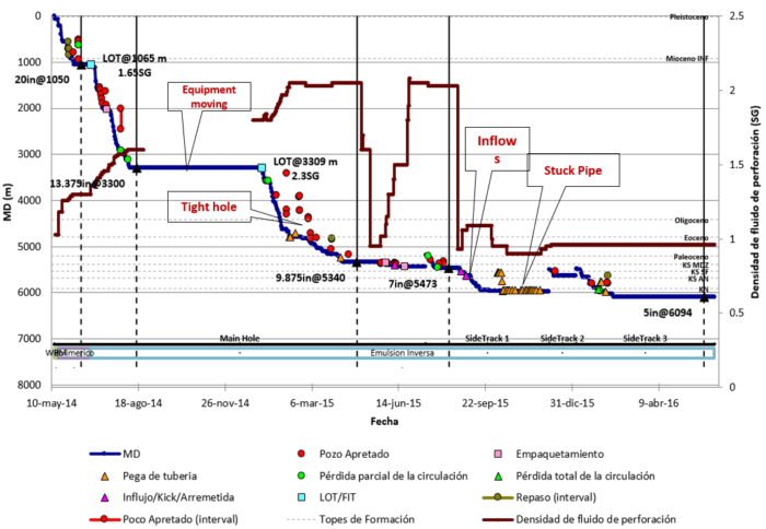
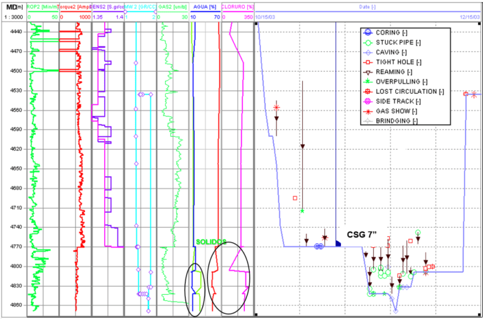
The Drilling Event Analysis is a geomechanical evaluation of drilling data (most often, daily drilling report) in which we document: pore pressure indicators (e.g., gas inflows, kicks, and drill breaks); cuttings load and geometry; instability indicators (e.g., lost circulation – well was fractured or presence of natural fractures; tight hole; stuck pipe; high torque; reaming; excessive failure in the wellbore and excess cuttings volumes; and differential sticking); instantaneous or time dependent instability events; and operational or fluid-related well events.
These data are combined and evaluated in order to calibrate/validate the 1D geomechanical model and assist in a wellbore stability analysis.